Machine Learning for Pharmaceuticals | Blog Series | Part 2

Developing a Machine Learning Solution: The Case Example of Predictive Water Monitoring
In the previous blog post we provided the necessary information in order to create a basic understanding of the most common Artificial Intelligence concepts. Armed with this knowledge, the blog series will now shift its focus to a more practical point of view regarding the application of machine learning in a pharmaceutical environment. Always good to understand the theoretical principles, however real-life case examples are quite often a better way to capture the imagination.
As stated in the previous blog, the quality-focused nature of the pharmaceutical industry makes it a potentially valuable domain for discovering machine learning use-cases. Especially the business areas that are subjected to sampling procedures can instantly provide outcome data. When the outcome data is already available, the next logical step is to examine if potential input variables are directly obtainable. If available, or collection can start on short term, you have a potential opportunity that can be worth investigating. This investigation should be done cautiously and thorough, for example via a proof of concept.
For one of our customers we did the same, we identified an opportunity for the application of Artificial Intelligence and used the proof of concept methodology to determine the potential value. In this blog part we will reveal the process on how we came to the development of a predictive quality management solution: Predictive Water Monitoring. In order to be able to fully understand how we boiled down to the idea, it is required to understand some of the background of pharmaceutical water systems and to have an idea on how this sampling process is executed. Subsequently we will explain the inception of our idea for the proof of concept is explained, were we elaborate on how we connected the dots (or variables) that triggered us to develop a water-monitoring solution. Conclusively this blog will explain how we turned our discovery into a proof of concept with various components, where the statistical models are utilized within a conceptual solution that can benefit pharmaceutical companies in managing their water-monitoring strategies.
Status Quo in Water Monitoring
Obviously water quality is of vital importance in a pharmaceutical environment, for example to function as an ingredient or to be applied in cleaning/sterilizing activities. Therefore regulatory requirements force companies to be in control of their water quality parameters. This is called water-monitoring and requires to provide proof that the required water quality was attained.
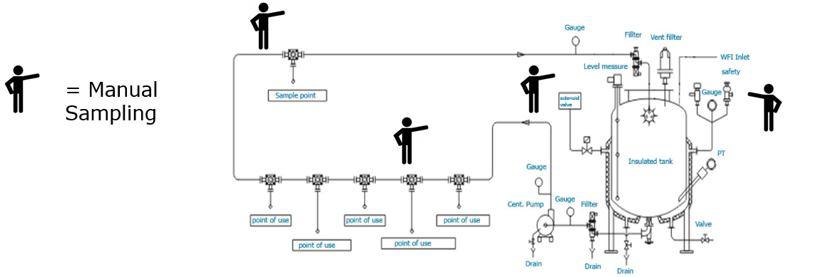
Figure 1: Example of water-loop in combination with the manual sampling process. (Click for more details)
Up until today the most common technique for water-monitoring is a manual sampling process, where, on an interval-based schedule all Points of Use (PoUs), supplying pharmaceutical grade water, are manually sampled with bottles. By the end of the sampling round, the sample bottles are handed over to the quality department which will then analyze the quality of the water via lab inspection. When the outcome of the sample analysis indicates that the quality of the water was not according to the required specification, the quality department is forced to start a quality investigation in order to determine its effects on final product quality. The result can for example be an additional lab test for of a production batch and/or a root-cause analysis on why the required water quality parameters were breached.
Unfortunately this process has multiple shortcomings. If we sum up the general downsides we can state that manual sampling: is cumbersome due to the amount time required in the collection and analysis of samples, is prone to a high probability of errors because of all the manual actions along the process, and is suboptimal since samples only provide a snapshot of the situation instead of providing insight in actual parametrical fluctuations over time.
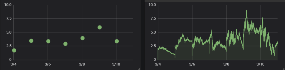
Figure 2: Graphical example of measuring Total Organic Carbon. These graphs illustrate the difference between periodic sampling (left) leading to a fragmented graph. Containg only ‘snapshots’ of the water quality, and monitoring the water quality continuously (right).
As can be seen, the periodic sampling procedure do not catch any fluctuations between sampling moments.
The Pharmaceutical Water Loop
Pharmaceutical water systems are set-up in so-called water loops. Due to the costly nature of producing pharmaceutical water, unused water along the loop is redistributed to a storage vessel, allowing it to be reused (if it still adheres to basic quality requirements), instead of being discharged directly into the sewer. Along this water loop various points of use (PoUs) and sample points exist, these can either be tap-points used in cleanrooms (e.g. for cleaning lab equipment) or direct connections to (critical) production machinery such as a bioreactors, separators and filling lines for pre-filled syringes.
All these PoUs and sample points require sampling and consecutive analysis on a daily basis, including the recording of results in a validated database to allow trend analysis which can help discover recurring, periodical fluctuations of certain parameters that influence the quality of the water. Ultimately, not adhering to the regulations resulting in the consumption of substandard water quality in the manufacturing process, can lead up to the rejection of the finished product.
To minimize this from happening, certain safeguarding instruments permanently monitoring the loop are deployed. Examples are: temperature sensors which can activate heat exchangers, in order to keep the loop at the right temperature and flow meters controlling circulation pumps, so the water keeps running.
Connecting the Dots (or Databases)
Our water-monitoring Eureka moment came at a moment when one of our customers approached us to help improve their current water monitoring strategies. The customer complained about the suboptimal and costly aspect of the manual sampling process and wondered if technological advances could bring any relief within the company. Obviously, this was the starting point of our investigation.
Armed with our understanding of the GMP industry and its regulations in combination with the knowledge of the technological possibilities, we started to examine the available data sources containing data on the water loop. As a starting point we had the database containing the lab results, and for some loops we even had the possibility to have direct insight on the critical water parameters such as measured by TOC analyzers, measuring the Total Organic Carbon (TOC) in the water loop.
Since there are numerous sensors on the water loop for safeguarding, we were also able to extract recorded sensor data and label this as the independent variables to be tested against the sample outcomes, to see if a statistical model with predictive capabilities can be generated. The typical independent variables that we were able to extract from these safeguarding instruments were: temperature, pressure, flow and conductivity. Combined with the sample outcomes, we were able to comprise a complete variable set. As a consequence, expert knowledge was required to understand if there are potential relationships between any of these discovered variables.
With the help of a lab analyst we found out that the majority of causes that lead to substandard water quality, can be caught in cause-effect relationships. Any activities along the water loop, such as sampling itself or maintenance activities, can bring the water quality out of balance. Other perfect examples of this cause-effect relationship: when the water temperature drops, bacterial growth such as legionella and endotoxins can be triggered, and a standstill of the water flow in the loop can lead to microbiological (or microbial) development such as algae or molds.
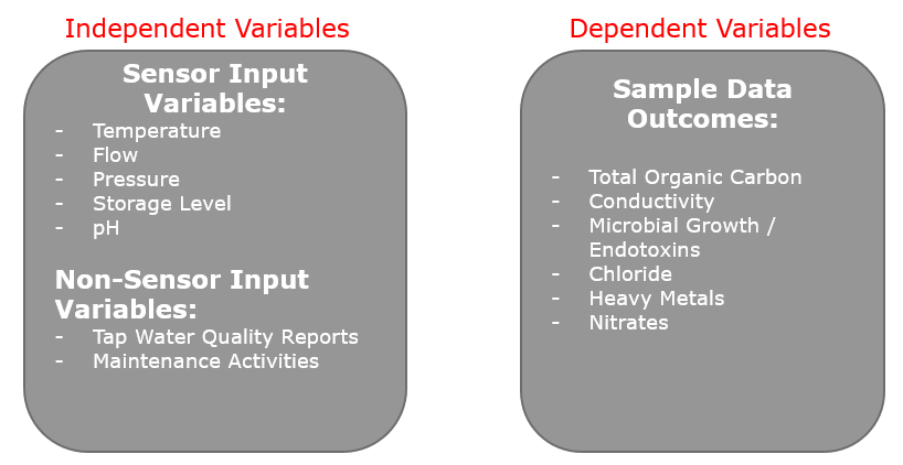
Figure 3: All collected variables that were utilized for the determination of relationships.
The identified relationships can be turned into statistical models allowing to provide for predictive capabilities on water quality.
Validating the Relationships
Based upon the identified variables and validated relationships, it was important to initially determine if significant relationships among independent and dependent variables could be identified. With the support of a data scientist, the data was prepared (cleansing) and various statistical modelling techniques were applied.
The results were promising: regression techniques exposed multiple relationships between the collected sensor data and sample outcome information. Furthermore by adding maintenance-related information (time, date, technical object and type of maintenance as registered in maintenance orders) from the ERP system, we could also confirm the impact of maintenance activities An interesting example is the high correlation between both temperature and pressure in relation to the amount of Total Organic Carbon (TOC) in the water-loop.
Proofing the Concept
Because the relationships among independent and dependent variables were mapped and validated, a machine learning solution could be established, since we are able to ‘predict’ the quality of the water. This final concept contains the following components:
- Ability to map a water-monitoring loop, including a possibility to link sensor data with various technical components on this water loop, indicating the relevant quality parameters and pre-specify variable thresholds for alarming purposes. Furthermore the components that were mapped in water-monitoring loop should be synchronized with the Laboratory Information Management System (LIMS) to include sample outcome data. By enriching the data with information form the Central Maintenance Management System (CMMS), maintenance order information could also be included to check for historical maintenance activities on the water-loop.
- Sample worklist, in order to improve accuracy on sample-taking. Since certain points still require sampling, a guided user interface should support the sample-taker in properly registering the samples. Not only a more accurate timestamp, but also the possibility to scan QR-/Bar-codes on sample bottles and sample points for linking purpose should reduce the error margin on sample data.
- Machine Learning Component, this final part brings all information together, including the possibility to maintain underlying statistical models (e.g. change variables or re-train model). In this part of the solution the statistical models allow to predict when the identified dependent variables will be going outside of their thresholds, based upon independent variable information. It is all combined in uncomplicated graphical overview allowing to check each of the variables, their relationships and to generate alarms based upon expected breaches of water quality.
These components were developed within our Proof of Concept. By only focusing on a single water loop in combination with small subset of variables, we were able to quickly develop the solution portfolio and to demonstrate the added value towards our customer in a tangible manner. Furthermore we never lost track of potential scalability. As in every successful Proof of Concept, the modular nature of the solution allows to quickly upscale and transform this concept into a complete IT component that can be utilized in multiple business processes.
Examples of the Graphical Machine Learning Component in Our PoC
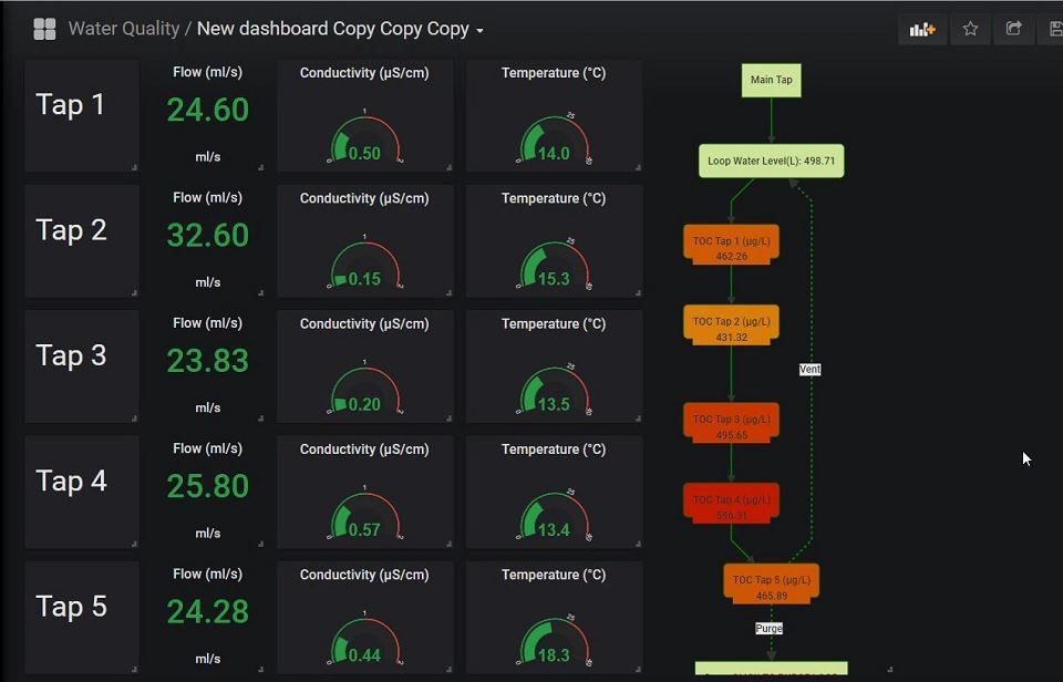
Figure 4: Overview of live sensor information, mapped along the water-loop in a graphical representation. The meters also contain threshold data, in order to indicate when important parameters are breached. All data in the overivew is updated every 5 seconds with fresh sensor information. (Click for more details)
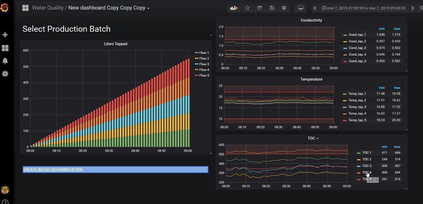
Figure 5: The ‘Production Batch Overview‘ allows QA departments to retrospectively check the water quality used in batch production. It also includes a functionality to generate batch report documenation containing the critical parameters of all water that was used in producing a specific batch. This allows QA departments to directly have insight and provide proof that relevant parameters were in control. (Click for more details)
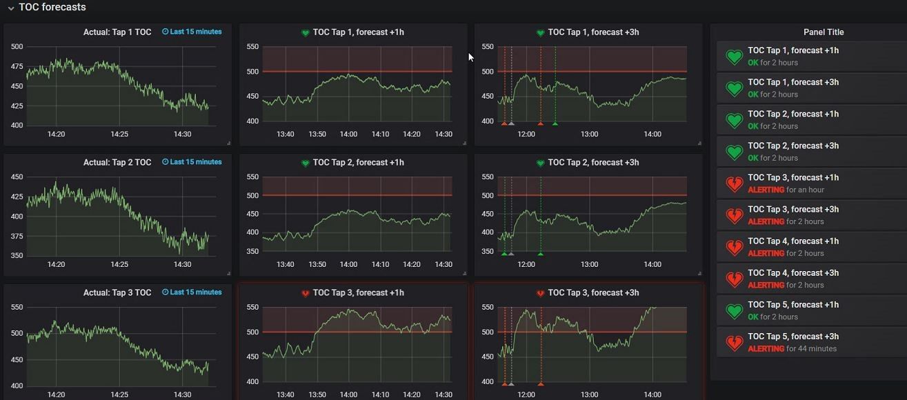
Figure 6: The holy grail of our solutin: the predictive dashboard. The charts on the left contain the historical data of a certain dependent variable, where the middle and right set of charts already predict the water quality. The middle row of charts can look 1 hour ahead, the right row even 3 hours in the future. On the far right of the screen you can see all generated alarms on the future quality of the water. This allows companies to anticipated on possible threshold breaches (e.g determine to postpone production of a batch until water parameters are in control). (Click for more details)
In the next and final blog, we will zoom-in on how you can start with implementing Artificial Intelligence solutions within your company. We discuss the ingredients and roadmap on how to move from idea, to proof of concept, and ultimately into a complete solution for the reinforcement of various business processes.
If you would like to know more about our water-monitoring solution, such as the IT components or statistical models that were utilized, or the final result of the complete water-monitoring portfolio, feel free to contact us. We are happy demonstrate the logic and capabilities of this solution.